Real life applications of mathematics
$$ \int { } $$
I actually used advanced maths once in my life. I dropped my keys in the toilet, so I had to use an integral-shaped wire to get them out.
I need your attention

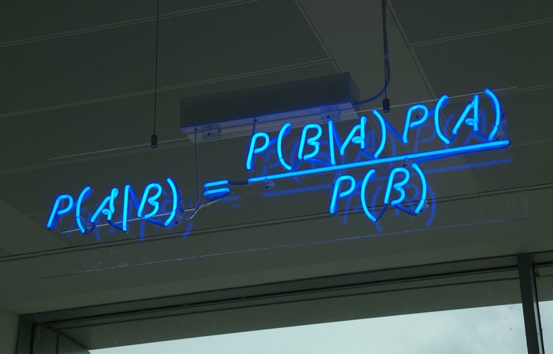
An Intuitive Explanation of
Bayes' Theorem

$$P\left( A \right) =\frac { \left| A \right| }{ \left| U \right| }$$ $$ P\left( \neg A \right) =1-P\left( A \right) $$
$$P\left( B \right) =\frac { \left| B \right| }{ \left| U \right| }$$ $$ P\left( \neg B \right) =1-P\left( B \right) $$
$$P\left( AB \right) =\frac { \left| AB \right| }{ \left| U \right| }$$
$$P\left( { A }|{ B } \right) =\frac { \left| AB \right| }{ \left| B \right| } =\frac { \frac { \left| AB \right| }{ \left| U \right| } }{ \frac { \left| B \right| }{ \left| U \right| } } =\frac { P\left( AB \right) }{ P\left( B \right) }$$ $$P\left( { B }|{ A } \right) =\frac { \left| AB \right| }{ \left| A \right| } =\frac { \frac { \left| AB \right| }{ \left| U \right| } }{ \frac { \left| A \right| }{ \left| U \right| } } =\frac { P\left( AB \right) }{ P\left( A \right) }$$
Independence
A,B independent:
$$ P\left( { A }|{ B } \right) =P\left( A \right), \quad P\left( { B }|A \right) =P\left( B \right)$$
$$ P\left( { A }|{ B } \right) =\frac { P\left( AB \right) }{ P\left( B \right) } =P\left( A \right) $$
$$ P\left( AB \right) =P\left( A \right) \cdot P\left( B \right) $$
Example of Independence
$$P\left( A \right) =0.6,\quad P\left( B \right) =0.5\\ P(AB)=0.6\cdot 0.5=0.3$$

- 1% of women in the group have breast cancer: $ P\left( A \right) =0.01 $
- 80% of women with breast cancer get a positive mammogram: $ P\left( { B }|{ A } \right) =0.8 $
- 9.6% of the women without breast cancer get a positive mammogram too: $ P\left( { B }|{ \neg A } \right) =0.096 $
- What is the chance of actually having breast cancer given a positive mammogram? $ P\left( { A }|{ B } \right) =? $
Text classification
using Naive Bayes
Document: $ d=\left< { { w }_{ 1 },{ w }_{ 2 },\dots ,{ w }_{ { n }_{ d } } } \right> $
Document space: $ d\in D $
Categories: $ C=\left\{ { c }_{ 1 },{ c }_{ 2 },\dots ,{ c }_{ j } \right\} $
Classification function: $$\gamma : D\rightarrow C$$
MAP: maximum a posteriori
$$ { c }_{ map }=\underset { c\in C }{ argmax } \quad P\left( { { c } }|{ d } \right) $$
Straight way approach
$$ P\left( { { c } }|{ d } \right) =\frac { P\left( { d }|{ c } \right) \cdot P\left( c \right) }{ P\left( d \right) } =\frac { P\left( { { w }_{ 1 },{ w }_{ 2 },\dots ,{ w }_{ { n }_{ d } } }|{ c } \right) \cdot P\left( c \right) }{ P\left( { w }_{ 1 },{ w }_{ 2 },\dots ,{ w }_{ { n }_{ d } } \right) } =\\ =\frac { P\left( { { w }_{ 1 } }|{ c } \right) \cdot P\left( { { w }_{ 2 } }|{ c,{ w }_{ 1 } } \right) \cdot \dots \cdot P\left( { { w }_{ { n }_{ d } } }|{ c,{ w }_{ 1 },{ w }_{ 2 },\dots ,{ w }_{ { n }_{ d }-1 } } \right) \cdot P\left( c \right) }{ P\left( { { w }_{ 1 } } \right) \cdot P\left( { { w }_{ 2 } }|{ { w }_{ 1 } } \right) \cdot \dots \cdot P\left( { { w }_{ { n }_{ d } } }|{ { w }_{ 1 },{ w }_{ 2 },\dots ,{ w }_{ { n }_{ d }-1 } } \right) } $$
$$ P\left( { e }_{ 1 },e_{ 2 },\dots ,{ e }_{ N } \right) =P\left( { { e }_{ 1 } } \right) \cdot P\left( { { e }_{ 2 } }|{ { e }_{ 1 } } \right) \cdot \dots \cdot P\left( { e_{ N } }|{ e_{ 1 },{ e }_{ 2 },\dots ,{ e }_{ N-1 } } \right) $$
Example 3.1
$$ P\left( { spam }|secret,sport \right) \propto \\ \propto P\left( { secret }|spam \right) \cdot P\left( sport|spam \right) \cdot P\left( spam \right) $$
$$ P\left( { secret }|spam \right) \cdot P\left( sport|spam \right) \cdot P\left( spam \right) = \\=\frac { 1 }{ 3 } \cdot \frac { 1 }{ 9 } \cdot \frac { 3 }{ 8 } =\frac { 1 }{ 72 } $$
$$ P\left( { secret }|ham \right) \cdot P\left( sport|ham \right) \cdot P\left( ham \right) = \\=\frac { 1 }{ 15 } \cdot \frac { 1 }{ 3 } \cdot \frac { 5 }{ 8 } =\frac { 1 }{ 72 } $$
$$ P\left( spam|secret,sport \right) =\frac { \frac { 1 }{ 72 } }{ \frac { 1 }{ 72 } +\frac { 1 }{ 72 } } =\frac { 1 }{ 2 } $$

Houston, we have a problem
$$ P\left( { spam }|today,is,secret \right) =? $$
$$ P\left( today|spam \right) \cdot P\left( is|spam \right) \cdot P\left( secret|spam \right) \cdot P\left( spam \right) =\\ =\frac { 0 }{ 9 } \cdot \frac { 1 }{ 9 } \cdot \frac { 3 }{ 9 } \cdot \frac { 3 }{ 8 } =0 $$
$$ P\left( today|ham \right) \cdot P\left( is|ham \right) \cdot P\left( secret|ham \right) \cdot P\left( ham \right) =\\ =\frac { 2 }{ 15 } \cdot \frac { 1 }{ 15 } \cdot \frac { 1 }{ 15 } \cdot \frac { 5 }{ 8 } =\frac { 1 }{ 2700 } $$
$$ P\left( spam|today,is,secret \right) =\frac { 0 }{ 0 +\frac { 1 }{ 2700 } } = {0} $$
Use the Laplace Smoothing, Luke
$ LS\left( k \right) $:
$$ P\left( x \right) =\frac { { N }_{ x }+k }{ N+k\cdot \left| X \right| } $$
LS(1)
| SPAM | HAM |
|---|---|
| offer is secret | play sport today |
| click secret link | went play sport |
| secret sport link | secret sport event |
| sport is today | |
| sport costs money |
$$ P\left( spam \right) =\frac { 3+1 }{ 8+2 } =\frac { 4 }{ 10 } ,\quad P\left( ham \right) =\frac { 5+1 }{ 8+2 } =\frac { 6 }{ 10 } $$
$$ P\left( { secret }|{ spam } \right) =\frac { 3 + 1 }{ 9 + 12 } =\frac { 4 }{ 21 } ,\quad P\left( { secret }|{ ham } \right) =\frac { 1 + 1 }{ 15 + 12 } =\frac { 2 }{ 27 }$$
$$ P\left( { sport }|{ spam } \right) =\frac { 1 + 1 }{ 9 + 12} = \frac { 2 }{ 21 },\quad P\left( { sport }|{ ham } \right) =\frac { 5 + 1 }{ 15 + 12 } =\frac { 2 }{ 9 } $$
Houston, we have no problem
$$ P\left( { spam }|today,is,secret \right) =? $$
$$ P\left( today|spam \right) \cdot P\left( is|spam \right) \cdot P\left( secret|spam \right) \cdot P\left( spam \right) =\\ =\frac { 1 }{ 21 } \cdot \frac { 2 }{ 21 } \cdot \frac { 4 }{ 21 } \cdot \frac { 2 }{ 5 } = \frac { 16 }{ 46305 } $$
$$ P\left( today|ham \right) \cdot P\left( is|ham \right) \cdot P\left( secret|ham \right) \cdot P\left( ham \right) =\\ =\frac { 1 }{ 9 } \cdot \frac { 2 }{ 27 } \cdot \frac { 2 }{ 27 } \cdot \frac { 3 }{ 5 } =\frac { 4 }{ 10935 } $$
$$ P\left( spam|today,is,secret \right) =\frac { \frac { 16 }{ 46305 } }{ \frac { 16 }{ 46305 } +\frac { 4 }{ 10935 } } = \frac { 324 }{ 667 } $$
Demo #01
Solving the problem of floating point underflow
$$ { c }_{ map }=\underset { c\in C }{ argmax } \quad P\left( c \right) \cdot \prod _{ i=1 }^{ { n }_{ d } }{ P\left( { { w }_{ i } }|{ c } \right) } $$
It's better to perform the computation by adding logarithms of probabilities instead of multiplying probabilities.
$$ \log { \left( x\cdot y \right) =\log { \left( x \right) } } +\log { \left( y \right) } $$
$$ { c }_{ map }=\underset { c\in C }{ argmax } \quad \left[ \log { \left( P\left( c \right) \right) +\sum _{ i=1 }^{ { n }_{ d } }{ \log { \left( P\left( { { w }_{ i } }|{ c } \right) \right) } } } \right] $$
Improving text classification
using feature selection
Confusion matrix
for a binary classifier
| Actual value | |||
|---|---|---|---|
| positive (TP+FN) |
negative | ||
Predicted value |
positive (TP+FP) |
True positive (TP) |
False positive (FP) |
| negative | False negative (FN) |
True negative (TN) |
|
Precision
$$ Precision=P\left( { actual\quad positive }|{ predicted\quad positive } \right) $$ $$ =\frac { TP }{ TP+FP } $$
Recall/Sensitivity
$$ Recall=P\left( { predicted\quad positive }|{ actual\quad positive } \right) $$ $$ =\frac { TP }{ TP+FN } $$
Precision vs. Recall
- You can always get a recall of 1 (but very low precision) by doing positive prediction for all documents
- Usually precision decreases as the number of positive predictions is increased
F-measure
$$ F=\frac { 1 }{ \alpha \frac { 1 }{ P } +(1-\alpha )\frac { 1 }{ R } } =\frac { ({ \beta }^{ 2 }+1)PR }{ { \beta }^{ 2 }P+R } $$
where
$ \quad { \beta }^{ 2 }=\frac { 1-\alpha }{ \alpha } $
$ \quad \alpha \in [0,1] $ and thus $ \beta \in [0,\infty ] $
Balanced F-measure
$$ { F }_{ 1 }={ F }_{ \beta =1 }=\frac { 2PR }{ P+R } $$
- The harmonic mean is always less than or equal to the arithmetic mean and the geometric mean
- When the values of two numbers differ greatly, the harmonic mean is closer to their minimum than to their arithmetic mean
Combinatorial Entropy
Multinomial coefficient: $$ W=\frac { N! }{ \prod { { N }_{ i }! } } =\frac { 10! }{ 5!\cdot 3!\cdot 2! } $$
Combinatorial entropy: $${ S }_{ comb }=\frac { \log _{ 2 }{ W } }{ N } =\frac { 1 }{ N } \log _{ 2 }{ \left( \frac { N! }{ \prod { { N }_{ i }! } } \right) } $$
Shannon entropy
$ { S }_{ comb }=\frac { 1 }{ N } \log _{ 2 }{ \left( \frac { N! }{ \prod { { N }_{ i }! } } \right) } =\frac { 1 }{ N } \left( \log _{ 2 }{ \left( N! \right) } -\log _{ 2 }{ \left( \prod { { N }_{ i }! } \right) } \right) $
Stirling's approximation: $$ \ln { \left( N! \right) } =N\ln { \left( N \right) } -N+O\left( \ln { \left( N \right) } \right) \approx n\ln { \left( n \right) } -n $$
$$ { S }_{ comb }\approx -\sum { \left( \frac { { N }_{ i } }{ N } \log _{ 2 }{ \left( \frac { { N }_{ i } }{ N } \right) } \right) } =-\sum { { p }_{ i }\log _{ 2 }{ { p }_{ i } } } $$
Entropy and
Mutual Information
$$ H(X)=-\sum _{ x\in X }^{ }{ p(x)\log _{ 2 }{ p(x) } } $$
The conditional entropy of X given Y is denoted: $$ H\left( { X }|{ Y } \right) =-\sum _{ y\in Y }^{ }{ p(y) } \sum _{ x\in X }^{ }{ p\left( { x }|{ y } \right) \log _{ 2 }{ p\left( { x }|{ y } \right) } } $$
Mutual Information between X and Y: $$ I(X;Y)=H(X)-H\left( { X }|{ Y } \right) $$
$$ =\sum _{ x\in X }^{ }{ \sum _{ y\in Y }^{ }{ p(xy)\log _{ 2 }{ \frac { p(xy) }{ p(x)p(y) } } } } $$
Mutual Information of
term and class
$$ I(U,C)=\sum _{ { e }_{ t }\in \left\{ 1,0 \right\} }^{ }{ \sum _{ { e }_{ c }\in \left\{ 1,0 \right\} }^{ }{ p(U={ e }_{ t },C={ e }_{ c })\log _{ 2 }{ \frac { p(U={ e }_{ t },C={ e }_{ c }) }{ p(U={ e }_{ t })p(C={ e }_{ c }) } } } } $$
$ { e }_{ t }=1 $ - the document contains term t
$ { e }_{ t }=0 $ - the document does not contain t
$ { e }_{ c }=1 $ - the document is in class c
$ { e }_{ c }=0 $ - the document is not in class c
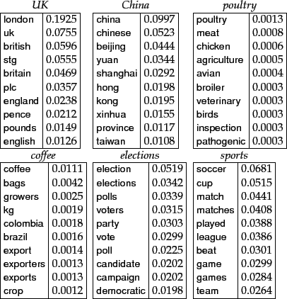
Features with high mutual information scores for six Reuters-RCV1 classes
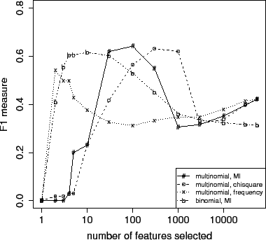
Effect of feature set size on accuracy for multinomial and Bernoulli models
- w - original word
- c - correction
We are trying to find the correction c, out of all possible corrections, that maximizes the probability of c given the original word w:
$$ { argmax }_{ c }\quad P\left( { c }|{ w } \right) $$
By Bayes' Theorem:
$$ { argmax }_{ c }\quad P\left( { c }|{ w } \right) =\\ ={ argmax }_{ c }\quad P\left( { w }|c \right) \cdot P\left( c \right) $$
- $ P\left( c \right) $ - the probability that a proposed correction c stands on its own.
- $ P\left( { w }|c \right) $ - the probability that w would be typed in a text when the author meant c.
The possible corrections c of a given word w
- Deletion (remove one letter)
- Transposition (swap adjacent letters)
- Alteration (change one letter to another)
- Insertion (add a letter)
For a word of length $n$, there will be $n$ deletions, $n-1$ transpositions, $26\cdot n$ alterations, and $26\cdot \left( n+1 \right)$ insertions, for a total of $54\cdot n+25$ (of which a few are typically duplicates).
The literature on spelling correction claims that 80% to 95% of spelling errors are an edit distance of 1 from the target.
Model assumptions
All known words of edit distance 1 are infinitely more probable than known words of edit distance 2, and infinitely less probable than a known word of edit distance 0.
$$ P\left( { { c }_{ 0 } }|{ w } \right) \gg P\left( { { c }_{ 1 } }|{ w } \right) \gg P\left( { { c }_{ 2 } }|{ w } \right) $$
$$ P\left( { 'word' }|{ 'word' } \right) \gg \\ \gg P\left( { 'world' }|{ 'word' } \right) \gg \\ \gg P\left( 'bored'|{ 'word' } \right) $$
What would Bayes say?
$$ P\left( { { c }_{ 0 } }|{ w } \right) \gg P\left( { { c }_{ 1 } }|{ w } \right) \gg P\left( { { c }_{ 2 } }|{ w } \right) $$
$$ \frac { P\left( { w }|{ { c }_{ 0 } } \right) \cdot P\left( { c }_{ 0 } \right) }{ P\left( w \right) } \gg \frac { P\left( { w }|{ { c }_{ 1 } } \right) \cdot P\left( { c }_{ 1 } \right) }{ P\left( w \right) } \gg \frac { P\left( { w }|{ { c }_{ 2 } } \right) \cdot P\left( { c }_{ 2 } \right) }{ P\left( w \right) } $$
$$ P\left( { w }|{ { c }_{ 0 } } \right) \cdot P\left( { c }_{ 0 } \right) \gg P\left( { w }|{ { c }_{ 1 } } \right) \cdot P\left( { c }_{ 1 } \right) \gg P\left( { w }|{ { c }_{ 2 } } \right) \cdot P\left( { c }_{ 2 } \right) $$
Correction
$$ \underset { { c }_{ i }\in { E }_{ i }\left( w \right) }{ argmax } \quad P\left( { { c }_{ i } }|{ w } \right) =\\ =\underset { { c }_{ i }\in { E }_{ i }\left( w \right) }{ argmax } \quad P\left( { w }|{ c }_{ i } \right) \cdot P\left( { c }_{ i } \right) =\\ =\underset { { c }_{ i }\in { E }_{ i }\left( w \right) }{ argmax } \quad P\left( { c }_{ i } \right) =\\ =\underset { { c }_{ i }\in { E }_{ i }\left( w \right) }{ argmax } \quad { N }_{ { c }_{ i } } $$
${ E }_{ i }\left( w \right)$ - all known words of edit distance $i$
Demo #02

|
|